
 This post was in the works for over a month. The chalk happened in one evening, but the research and writing took time. Taylor series make for a meaty topic, and Brook Taylor had a full life. Plus, infinity took me on a few tangential journeys.
The big idea here is approximation, in particular the evolution of methods involving infinite series like we saw in π and Powers of One Half. Enjoy!
In this age of hand-held devices with the raft of useful and sometimes frighteningly “necessary” apps, it can be easy to forget what it may have been like to do math by hand.
My calculus students worked a fair number of problems by hand, but they also used their TI-8*’s to graph and evaluate trig functions, evaluate derivatives, and calculate the volumes of solids of revolution. Every once in a while, a student would ask, “But, how does my calculator compute the value of sin(π/4)? Or, even π for that matter?”
Good question.
 I can tell you Newton had it right when he said he was standing on the shoulders of giants. The game of approximating transcendental values with ever-improving elementary iterations was established over 2200 years ago in Sicily. The ever-insightful Archimedes used several straight lines to approximate a circle and thereby approximate the value of π, the ratio of the circumference of any circle to its diameter.
In the 17th century, mere decades before Newton and Leibniz were born, Kepler is said to have built on Archimedes’ work using infinitesimals: numerical quantities so small there is no hope of seeing or measuring them. Kepler was working on finding the area of the circle, as opposed to the circumference.[1] He began with one of Archimedes’ polygons and then let the number of sides head off to infinitely. Thus, each side shrunk to an infinitely small length, an infinitesimal, and the polygon “became” a circle. Kepler’s work along with that of many others laid the foundation for Leibniz and Newton to work their seeming magic. Good job, Kepler.
The birth of calculus was not the end of approximation. It was a new beginning. At the turn of the 18th century, when calculus was barely crawling under the heavy load of notation and arguments for primacy, mathematicians were at work developing and improving approximation methods. All with a new conception of infinity on its way.[2]
 Millennia after Archimedes approximated π, Brook Taylor introduced the world to a new species of infinite series. Taylor’s polynomials gave us a way to approximate not just a number, like π, but a function itself: a function like ex or sin x.[3]
Don’t be scared off by the phrase, “infinite series.” You saw an infinite series in a recent post when we added up powers of one-half. I suppose you can be scared, but have some courage, too. Read on. It’ll be okay.
Brook Taylor, born in 1685, was an Englishman. He loved music and painting. A few years shy of his thirtieth birthday, he joined The Royal Society. In 1712, Taylor joined the committee investigating the conflict over who invented calculus.[4] In one corner a German philosopher and mathematician and in the other an English physicist and mathematician. Would you like to guess who the Royal Society of London favored?
If you think doing math is challenging (It is, for sure, for all of us at some point), imagine trying to accomplish something profound amidst a dispute between the mathematicians of England (your friends and teachers) and the greats emerging in continental Europe. (For my younger readers: It’s probably like trying to do homework while your parents are arguing. Not easy, right?) Taylor was working during the same epoch as Newton in England, while folks like the Bernoulli brothers, Johann and Jacob, were establishing “the Continent” as a powerhouse of mathematics.[5]
In 1715, Taylor published a paper with what would become known as Taylor Series. His paper, Methodus Incrementorum Directa et Inversa, is available online.[6] Taylor, like those before and after him, made discoveries in the rich soil of his predecessors’ findings and the (sometimes heated) dialogues with contemporaries. James Gregory, Newton, Leibniz, Johann Bernoulli, and Abraham de Moivre worked with series expansions of functions. Years later, Taylor’s theorem about series expansions gained importance when Euler and Lagrange put it to work.[7]
As you may have seen before, a series is the sum of a sequence of numbers. A power series is, “A sum of powers of a variable. A power series is essentially an infinite polynomial.” (Wolfram Alpha) Here is a simple one.

The ellipsis means just what we expect: continue the terms with larger and larger exponents. Forever. This power series is a Taylor series. A finite number of the terms, something like

approximates the following function near x = 0.[8]

With the ellipsis, and thereby all infinitely many terms, the Taylor series equals the function.

Why is 1 + x + x2 + x3 + … a Taylor series? It follows the rule Taylor outlined in his paper. His rule, called the Taylor theorem, says a function, f (x), can be represented by a polynomial where the coefficients are determined by evaluating the function and its derivatives at a particular x-value.[9] Here is the modern notation for Taylor series.

This is a formula of sorts. Choose values to plug in and a polynomial arises where the only variable is x. Those bits that look like apostrophes in the formula can be read as “prime.” They indicate derivatives of the function f. The exclamation marks indicate factorial. “3!” is read “three factorial.”

If you know a little calculus, I encourage you to build the Taylor series for 1/(1 – x). Rewrite f (x) as (1 – x)-1, and use a = o. Then watch the power rule for derivatives wipe out those factorials.
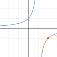
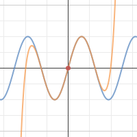
A Taylor series for a function can be found for any value of a. The value of a controls where the approximation is centered. If a = 2, then the polynomial approximates the function around 2 on the x-axis. The graph shows a Taylor polynomial up to the fourth power (with an x4 term) approximating the function 1/(1 – x) around 2. That orange curve is not doing too badly as an approximation of the blue one, when x is close to 2 at least.
When a = 0, the series is known as a Maclaurin series. This special case is named for the Scottish mathematician Colin Maclaurin. He was born in 1698, began university studies in Glasgow when he was 11, and became a professor of mathematics at the age of 19. Precocious? Yes, I should say so. When Maclaurin was 20, he met Newton and proceeded to expand the field of calculus. (Wikipedia)


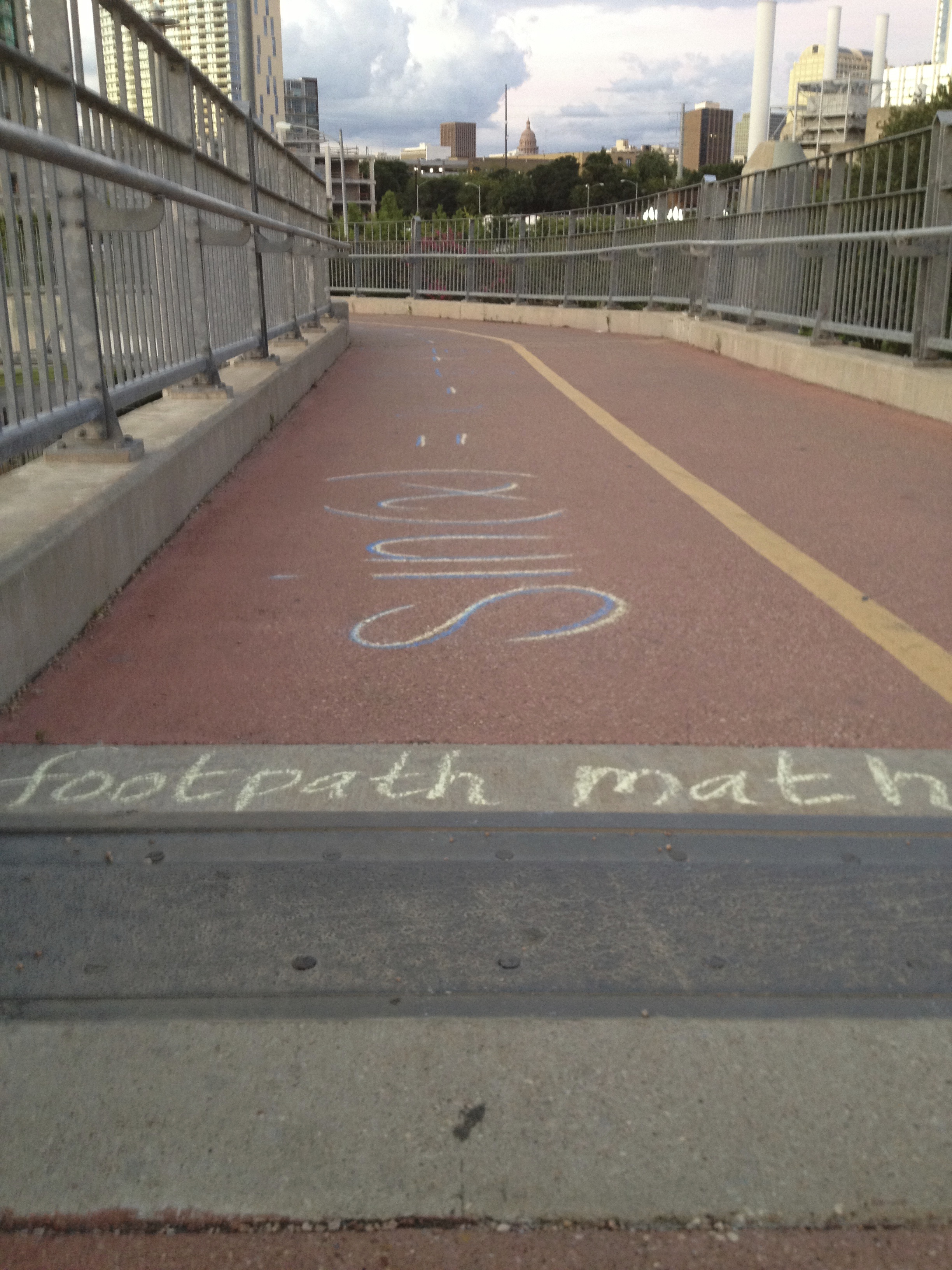
The series that found its way onto Austin pavement was a Maclaurin series for sin(x). Let’s see how the series comes into being. Using the formula for a Taylor series from above and setting a to zero, we get
To get our sine series from here, we will:
- Use sin(x) for f (x).
- Find the first, second, third (and so on) derivatives.
- Evaluate those derivatives at 0.
- Build our power series with the coefficients f (n)(0)/n!


I am going to share a few intermediate steps and leave some details to your imagination. Following the steps outlined above, we would see

Then, all of the sine terms disappear, since sin(0) = 0, and since cos(0) = 1,
with the pattern continuing indefinitely. The signs of the remaining terms alternate due to the nature of the relationship between sine and cosine.
The polynomial of 5 terms ending with x to the ninth, is not a bad approximation of sin(x). The graph to the right shows the Taylor polynomial and sin(x) itself.
The tale of Brook Taylor is not quite over. Taylor published the paper with what would become known as Taylor’s theorem and Taylor series in 1715 around the age of 30. Six years later, Taylor’s personal life began to unravel.
In that year he married Miss Brydges from Wallington in Surrey. Although she was from a good family, it was not a family with money and Taylor’s father strongly objected to the marriage. The result was that relations between Taylor and his father broke down and there was no contact between father and son until 1723. It was in that year that Taylor’s wife died in childbirth. The child, which would have been their first, also died. (MacTutor Archive)
Over the following six years, Taylor married and lost a second wife to childbirth. His relationship with his father was restored upon the second marriage, but Taylor was to lose his father just a year before his second wife, Sabetta, passed away. Their daughter, Elizabeth survived.
Sometimes, I envy the lives of mathematicians living and working in the 18th and 19th centuries. Liberty, equality and fraternity were altering the face of government in France. And, so many exciting mathematical discoveries were made! Mostly though, I am grateful to live and work in the era of the silicon chip, refrigeration, mobile phones, and health care based on science and reason.


1.^ Kepler was very interested in area. What is now known as Kepler’s Second Law involves the motion of planets and the areas they sweep out in time. Equal time will result in equal area. Read and see more about Kepler’s laws in the Physics Classroom.
2.^ Our conception of infinity changed dramatically in the 19th century. Cauchy, of whom we will have to hear more, reformulated the theoretical underpinnings of calculus. Then, Weierstrass, Dedekind, and Cantor did away with infinitesimals and reframed how mathematicians perceive numbers:
… a nominalistic reconstruction successfully implemented at the end of the 19th century by Cantor, Dedekind, and Weierstrass. The rigorisation of analysis they accomplished went hand-in- hand with the elimination of infinitesimals; indeed, the latter accomplishment is often viewed as a fundamental one. (Katz and Katz 16)
Karin Usadi Katz and Mikhail G. Katz (2011) A Burgessian Critique of Nominalistic Tendencies in Contemporary Mathematics and its Historiography. Foundations of Science. See arxiv.
3.^ You have seen sine before. The sine of an angle is the ratio of the length of opposite leg to the length of the hypotenuse.

4.^ The MacTutor History of Math archive is a great resource. The pages on Brook Taylor gave me a valuable glimpse into his life, both personal and professional.
More information on the different motivations and perspectives held by Newton and Leibniz in the creation of calculus can be found in the archive.
5.^ For the better part of a century, from the late 1600s to the late 1700s, the Bernoulli family was producing mathematicians. From Bernoulli’s principle, named for Daniel who studied hydrodynamics, to Bernoulli numbers, named for Jacob, Daniel’s uncle, who founded the calculus of variations with his brother, Daniel’s father, Johann. Johann was also Euler’s PhD advisor! Check out Wikipedia’s Bernoulli Family page for more on this prolific lineage. And, check out the Mathematics Genealogy Project page on Euler to see a different kind of lineage.
6.^ Look for Proposition VII, Theorem 3, Corollary 2. That is where you can find, though hard to interpret, a Taylor series. Scans of Taylor’s paper in Latin are available in Google Play, with Proposition VII, Theorem III, Corollary II found here.
There is a translated and annotated version from Ian Bruce at 17centurymaths.com. You’ll want this one.
Also, A Source Book in Mathematics 1200–1800 (Cambridge, Massachusetts: Harvard University Press, 1969), pages 329–332 have the paper translated into English in D. J. Struik. This source is mentioned on the Wikipedia Taylor series page.
7.^ I am grateful for the work of the School of Mathematics and Statistics at the University of St Andrews, Scotland. They are the keepers of The MacTutor History of Math archive.
8.^ We actually played with this idea in the last post. If you let x = 1/2, you get

 And, when I said “near,” I meant it. I mean x has to be less than 1 unit away from zero.
9.^ The derivative of a function is the instantaneous rate of change of the y-values with respect to the x-values. Here is good way to wrap your head around the idea. If you are in a car that is heading down a highway, you are getting farther away from wherever you left. Your distance is a function of time. As time passes, you get further away, i.e. the distance increases. Let’s call this function f (t). The first derivative of your distance function, denoted as f ‘(t), is the rate the distance is changing with respect to time, i.e. your speed (velocity is a better word). The second derivative would indicate whether your velocity was changing. We call that acceleration. So, f ”(t) would be your acceleration.
Another thing to note is the general form for the Taylor series can be written using sigma notation as

Real pretty, huh?
Also, before heading back to the post, keep in mind
Finite number of terms → Taylor polynomial → approximates the function
Infinitely many terms → Taylor series → equals the function
And, if you want a more mathy tutorial resource, check out Paul’s Online Math Notes. These notes are courtesy of a professor from Lamar University a member of the Texas State University System.
P.S. Kudos to you for making it this far. Good show!
P.P.S. Thanks go to Jaclyn for the encouragement and photography. She also had the brilliant idea of using the spiral walkway to capture the experience of the infinitude of a Taylor series.

I love teaching Taylor Series – especially the error analysis when using Taylor Polynomials to approximate functions. Thanks for another interesting post !
You are welcome! I am glad to know you are out there teaching Taylor series. I am slowly but surely coming around to appreciating approximation and error. Finding “the right answer” just might involve an iterative search, a series of approximations. Maybe someday I will make friends with big O and the error function.
I totally understood every bit of that.
This past spring, I went to see an exhibit of Picasso’s work at the Museum of Fine Arts in Houston. I think it was the first time I understood any bit of his work. Even the brief epiphanic experience has stayed with me. (Did I just imply my blog posts are in some way comparable to Picasso’s work? No… I shouldn’t do that. Should I?)
This piece was commissioned by George I, to be performed on the Thames. If Taylor wasn’t there, he probably heard about it…
Very nice. I like to think of you and others listening while reading this post.
I especially enjoyed the photographs, with the moody lighting. The size of the exponents surprised me. How long did it take to install?
Austin was looking pretty special that night. According to the photographic record, it took about 45 minutes. It felt longer than that… in a good way.